[1] 4.14
[1] 6.28
[1] 1.772005
[1] 1.144223
[1] 9.8596
PLS 206 — Applied Multivariate Modeling
UC Davis
2026-01-01
Free & open source
Used by ecologists, geneticists, agronomists, and data scientists worldwide
10,000+ packages on CRAN for specialized analyses
Reproducible science
Your entire analysis is a script — share it, re-run it, tweak it
What we’ll use R for this quarter:
Run code: Cmd+Enter (Mac) / Ctrl+Enter (Windows)
[1] 4.14
[1] 6.28
[1] 1.772005
[1] 1.144223
[1] 9.8596
Note
Use <- for assignment. Use = only inside function arguments.
[1] 2 4 6 8 10 20
[1] 4 5 10
[1] "banana"
[1] 4 5 10
[1] 4 5 10
[1] TRUE FALSE FALSE TRUE
[1] "apple" "grape"
[1] 42
[1] "hello"
'data.frame': 4 obs. of 3 variables:
$ rep : num 1 2 3 4
$ treat: chr "A" "B" "A" "B"
$ value: num 10.2 8.5 11.1 9.3
[1] 10.2 8.5 11.1 9.3
rep treat value
1 1 A 10.2
rep treat value
1 1 A 10.2
3 3 A 11.1
rep treat value log_value
Min. :1.00 Length:4 Min. : 8.500 Min. :2.140
1st Qu.:1.75 Class :character 1st Qu.: 9.100 1st Qu.:2.208
Median :2.50 Mode :character Median : 9.750 Median :2.276
Mean :2.50 Mean : 9.775 Mean :2.275
3rd Qu.:3.25 3rd Qu.:10.425 3rd Qu.:2.344
Max. :4.00 Max. :11.100 Max. :2.407
'data.frame': 178 obs. of 14 variables:
$ Cultivar : chr "barolo" "barolo" "barolo" "barolo" ...
$ Alcohol : num 14.2 13.2 13.2 14.4 13.2 ...
$ AlcAsh : num 15.6 11.2 18.6 16.8 21 15.2 14.6 17.6 14 16 ...
$ Ash : num 2.43 2.14 2.67 2.5 2.87 2.45 2.45 2.61 2.17 2.27 ...
$ Color : num 5.64 4.38 5.68 7.8 4.32 6.75 5.25 5.05 5.2 7.22 ...
$ Flav : num 3.06 2.76 3.24 3.49 2.69 3.39 2.52 2.51 2.98 3.15 ...
$ Hue : num 1.04 1.05 1.03 0.86 1.04 1.05 1.02 1.06 1.08 1.01 ...
$ MalicAcid : num 1.71 1.78 2.36 1.95 2.59 1.76 1.87 2.15 1.64 1.35 ...
$ Mg : int 127 100 101 113 118 112 96 121 97 98 ...
$ NonFlavPhenols: num 0.28 0.26 0.3 0.24 0.39 0.34 0.3 0.31 0.29 0.22 ...
$ OD : num 3.92 3.4 3.17 3.45 2.93 2.85 3.58 3.58 2.85 3.55 ...
$ Phenols : num 2.8 2.65 2.8 3.85 2.8 3.27 2.5 2.6 2.8 2.98 ...
$ Proa : num 2.29 1.28 2.81 2.18 1.82 1.97 1.98 1.25 1.98 1.85 ...
$ Proline : int 1065 1050 1185 1480 735 1450 1290 1295 1045 1045 ...
Cultivar Alcohol AlcAsh Ash Color Flav Hue MalicAcid Mg NonFlavPhenols
1 barolo 14.23 15.6 2.43 5.64 3.06 1.04 1.71 127 0.28
2 barolo 13.20 11.2 2.14 4.38 2.76 1.05 1.78 100 0.26
3 barolo 13.16 18.6 2.67 5.68 3.24 1.03 2.36 101 0.30
4 barolo 14.37 16.8 2.50 7.80 3.49 0.86 1.95 113 0.24
5 barolo 13.24 21.0 2.87 4.32 2.69 1.04 2.59 118 0.39
6 barolo 14.20 15.2 2.45 6.75 3.39 1.05 1.76 112 0.34
OD Phenols Proa Proline
1 3.92 2.80 2.29 1065
2 3.40 2.65 1.28 1050
3 3.17 2.80 2.81 1185
4 3.45 3.85 2.18 1480
5 2.93 2.80 1.82 735
6 2.85 3.27 1.97 1450
Tip
Always use str() after reading data — check that column types match what you expect.
[1] 150 5
Sepal.Length Sepal.Width Petal.Length Petal.Width
Min. :4.300 Min. :2.000 Min. :1.000 Min. :0.100
1st Qu.:5.100 1st Qu.:2.800 1st Qu.:1.600 1st Qu.:0.300
Median :5.800 Median :3.000 Median :4.350 Median :1.300
Mean :5.843 Mean :3.057 Mean :3.758 Mean :1.199
3rd Qu.:6.400 3rd Qu.:3.300 3rd Qu.:5.100 3rd Qu.:1.800
Max. :7.900 Max. :4.400 Max. :6.900 Max. :2.500
Species
setosa :50
versicolor:50
virginica :50
Pearson's product-moment correlation
data: iris$Sepal.Length and iris$Petal.Length
t = 21.646, df = 148, p-value < 2.2e-16
alternative hypothesis: true correlation is not equal to 0
95 percent confidence interval:
0.8270363 0.9055080
sample estimates:
cor
0.8717538
Save the result as an object and extract parts:
ggplot2 builds plots layer by layer:
ggplot(data, aes(x = ..., y = ...)) +
geom_*() + # geometry: points, lines, bars ...
labs() + # labels
theme_*() # styling
Every plot starts with ggplot() — then add layers with +
ggplot(iris,
aes(x = Sepal.Length,
y = Sepal.Width,
col = Species,
fill = Species)) +
geom_point(alpha = 0.7) +
geom_smooth(method = "lm", alpha = 0.1) +
labs(title = "Iris Dataset",
x = "Sepal Length (mm)",
y = "Sepal Width (mm)") +
scale_color_manual(values = c("gray30", "dodgerblue", "orange")) +
scale_fill_manual(values = c("gray30", "dodgerblue", "orange")) +
theme_classic(base_size = 14) +
theme(plot.title = element_text(face = "bold"),
legend.position = "top")
$ctrl
Min. 1st Qu. Median Mean 3rd Qu. Max.
4.170 4.550 5.155 5.032 5.293 6.110
$trt1
Min. 1st Qu. Median Mean 3rd Qu. Max.
3.590 4.207 4.550 4.661 4.870 6.030
$trt2
Min. 1st Qu. Median Mean 3rd Qu. Max.
4.920 5.268 5.435 5.526 5.735 6.310
Does the control group mean differ from 5.0 g?
One Sample t-test
data: ctrl
t = 0.17355, df = 9, p-value = 0.8661
alternative hypothesis: true mean is not equal to 5
95 percent confidence interval:
4.614882 5.449118
sample estimates:
mean of x
5.032
Non-parametric alternative:
Welch Two Sample t-test
data: x1 and x2
t = 1.1913, df = 16.524, p-value = 0.2504
alternative hypothesis: true difference in means is not equal to 0
95 percent confidence interval:
-0.2875162 1.0295162
sample estimates:
mean of x mean of y
5.032 4.661
Wilcoxon rank sum test with continuity correction
data: x1 and x2
W = 67.5, p-value = 0.1986
alternative hypothesis: true location shift is not equal to 0
95 percent confidence interval:
-0.2899731 1.0100554
sample estimates:
difference in location
0.4213948
Tip
Welch’s t-test is the safe default — it doesn’t assume equal variances.
Do all three treatment groups differ?
Df Sum Sq Mean Sq F value Pr(>F)
group 2 3.766 1.8832 4.846 0.0159 *
Residuals 27 10.492 0.3886
---
Signif. codes: 0 '***' 0.001 '**' 0.01 '*' 0.05 '.' 0.1 ' ' 1
Post-hoc pairwise comparisons:
Tukey multiple comparisons of means
95% family-wise confidence level
Fit: aov(formula = weight ~ group, data = PlantGrowth)
$group
diff lwr upr p adj
trt1-ctrl -0.371 -1.0622161 0.3202161 0.3908711
trt2-ctrl 0.494 -0.1972161 1.1852161 0.1979960
trt2-trt1 0.865 0.1737839 1.5562161 0.0120064
ggplot(PlantGrowth, aes(group, weight, fill = group)) +
geom_boxplot(alpha = 0.75, show.legend = FALSE) +
geom_jitter(width = 0.08, alpha = 0.6) +
labs(title = "Raw values (ANOVA)") +
theme_classic()
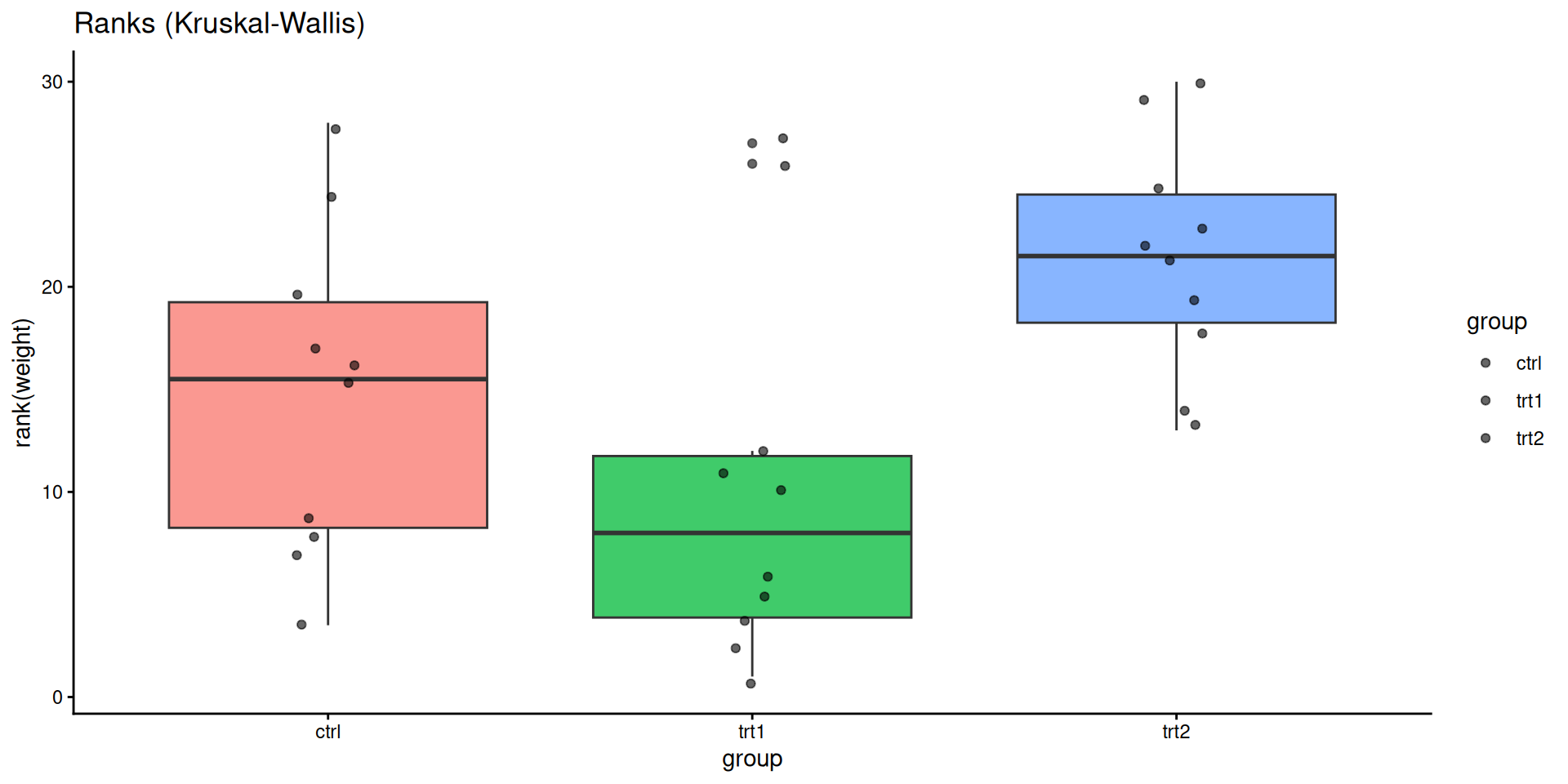
ggplot(PlantGrowth, aes(group, rank(weight), fill = group)) +
geom_boxplot(alpha = 0.75, show.legend = FALSE) +
geom_jitter(width = 0.08, alpha = 0.6) +
labs(title = "Ranks (Kruskal-Wallis)") +
theme_classic()

Kruskal-Wallis rank sum test
data: weight by group
Kruskal-Wallis chi-squared = 7.9882, df = 2, p-value = 0.01842
Pairwise follow-up with correction for multiple comparisons:
Pearson's product-moment correlation
data: sub$conc and sub$uptake
t = 4.3196, df = 19, p-value = 0.0003695
alternative hypothesis: true correlation is not equal to 0
95 percent confidence interval:
0.3910239 0.8709363
sample estimates:
cor
0.7038936
Spearman's rank correlation rho
data: sub$conc and sub$uptake
S = 256.28, p-value = 2.691e-06
alternative hypothesis: true rho is not equal to 0
sample estimates:
rho
0.8335869
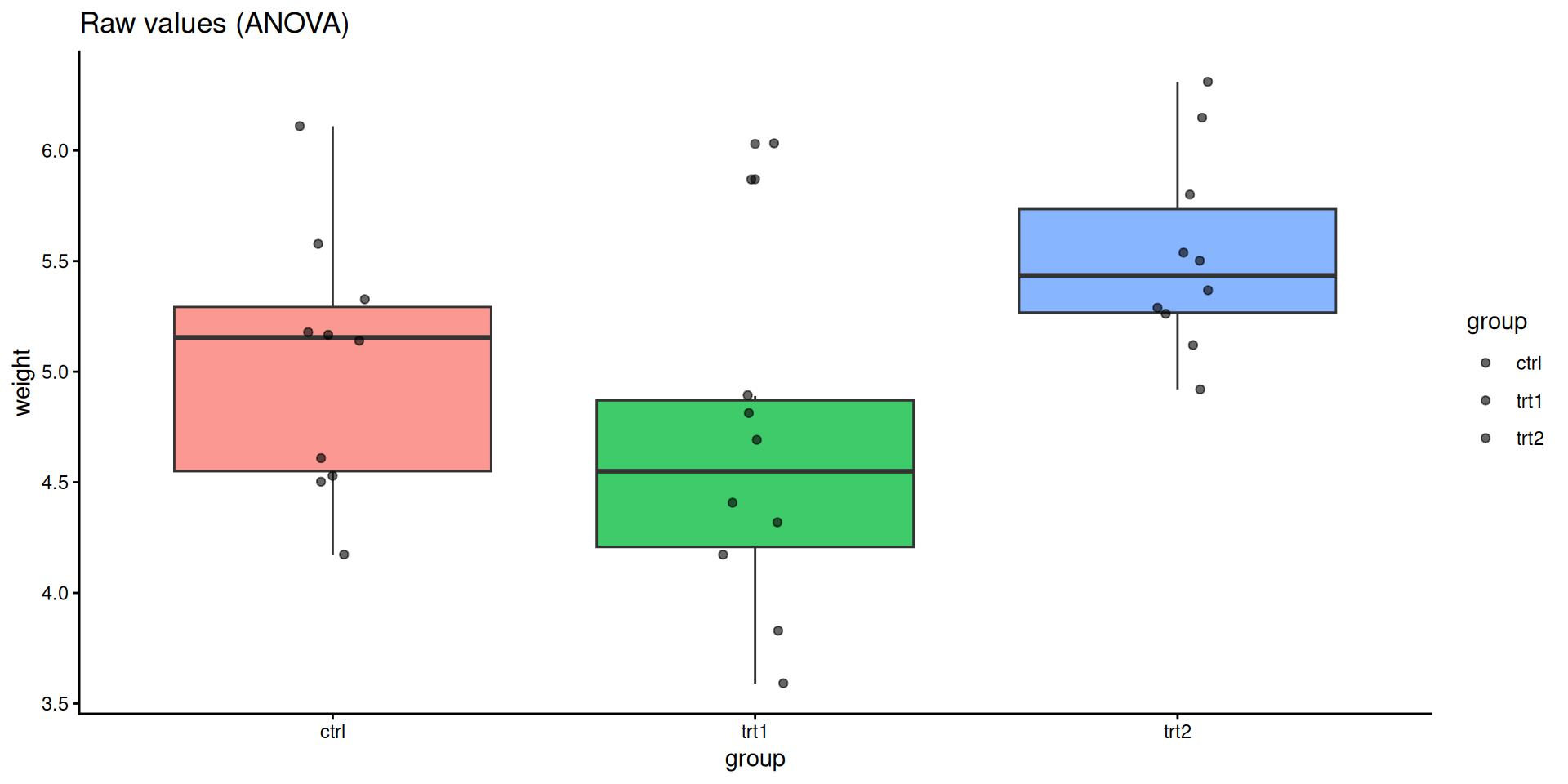
ggplot(sub, aes(conc, uptake)) +
geom_point() +
geom_smooth(method = "lm", linewidth = 0.8) +
geom_smooth(method = "loess", linetype = 2, linewidth = 0.8) +
labs(title = "Raw", x = "CO2 concentration", y = "Uptake") +
theme_classic()
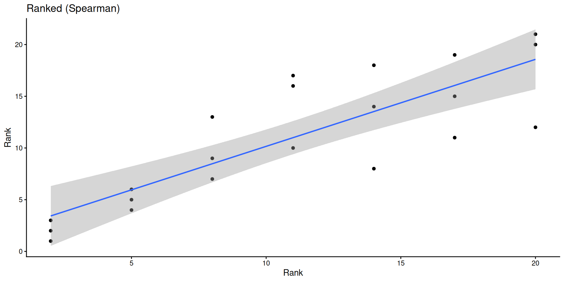
ggplot(sub, aes(rank(conc), rank(uptake))) +
geom_point() +
geom_smooth(method = "lm", linewidth = 0.8) +
labs(title = "Ranked (Spearman)", x = "Rank", y = "Rank") +
theme_classic()

Is pest presence associated with treatment?
Trt
Pest A B
Present 3 17
Absent 10 10
Fisher's Exact Test for Count Data
data: tab
p-value = 0.04074
alternative hypothesis: true odds ratio is not equal to 1
95 percent confidence interval:
0.02632766 0.94457354
sample estimates:
odds ratio
0.184812
Pearson's Chi-squared test
data: tab
X-squared = 5.584, df = 1, p-value = 0.01812
Tip
Use Fisher’s exact for small cell counts (any cell < 5). Use chi-squared for larger samples.
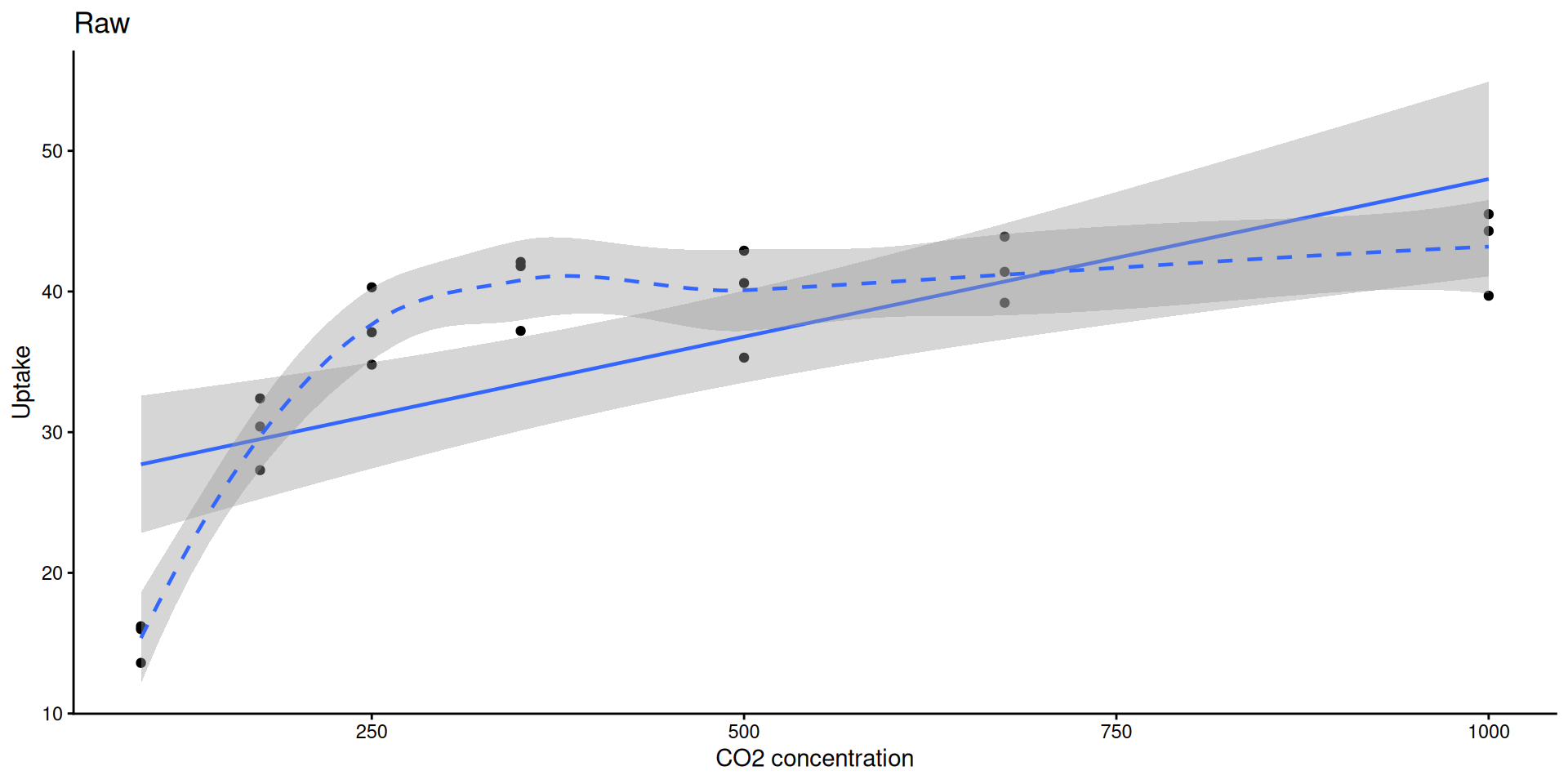
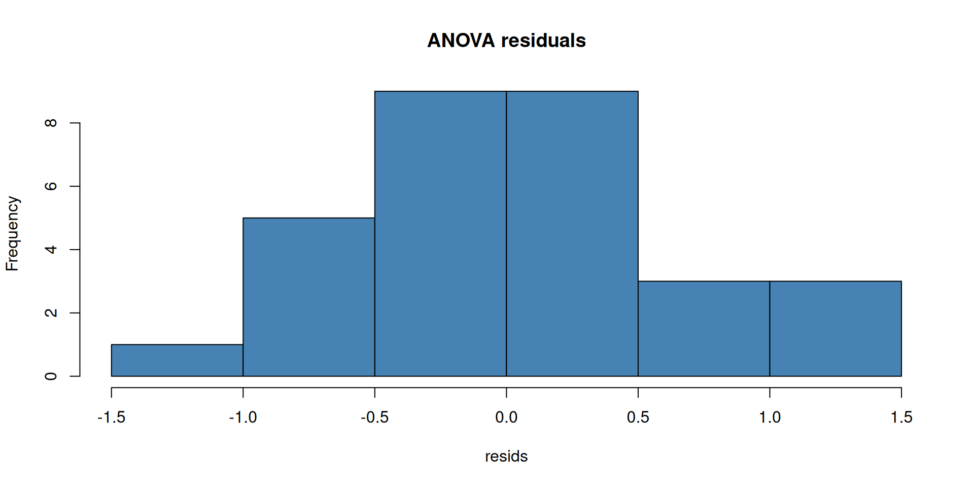
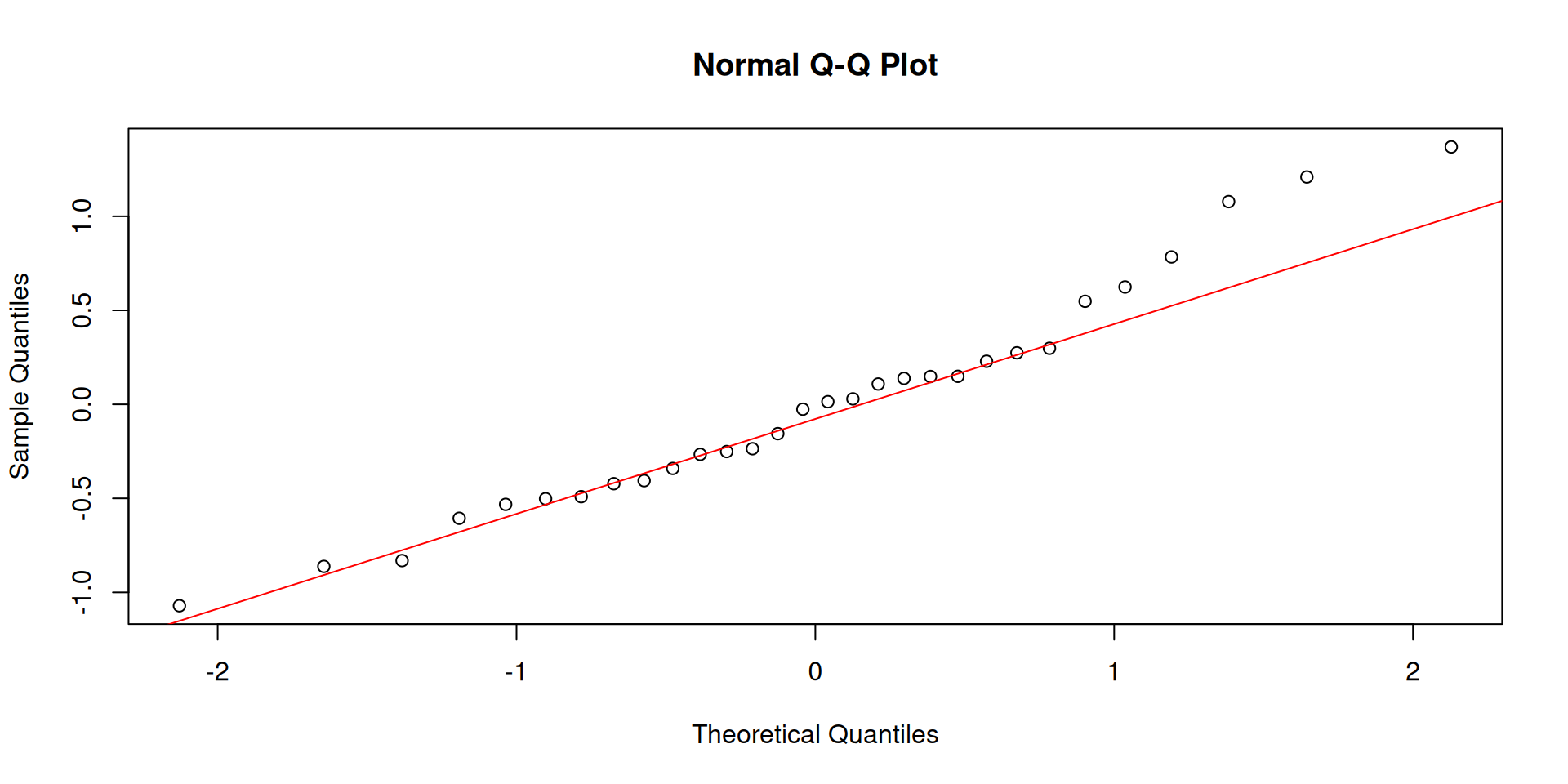
Always check your residuals, not the raw data:


Open the interactive page to explore these concepts live — no R needed:
Module 1 Interactive Explorers →
R foundations
Visualization
ggplot2: geom_point(), geom_smooth(), theme_classic()Statistics
Submit on Canvas.
Topics: reading data, basic data manipulation, a t-test, a correlation, and a simple ggplot.
Questions? Office hours Wednesday 9–10 AM (Zoom).
R version 4.4.3 (2025-02-28)
Platform: x86_64-pc-linux-gnu
Running under: Ubuntu 24.04.3 LTS
Matrix products: default
BLAS: /usr/lib/x86_64-linux-gnu/openblas-pthread/libblas.so.3
LAPACK: /usr/lib/x86_64-linux-gnu/openblas-pthread/libopenblasp-r0.3.26.so; LAPACK version 3.12.0
locale:
[1] LC_CTYPE=C.UTF-8 LC_NUMERIC=C LC_TIME=C.UTF-8
[4] LC_COLLATE=C.UTF-8 LC_MONETARY=C.UTF-8 LC_MESSAGES=C.UTF-8
[7] LC_PAPER=C.UTF-8 LC_NAME=C LC_ADDRESS=C
[10] LC_TELEPHONE=C LC_MEASUREMENT=C.UTF-8 LC_IDENTIFICATION=C
time zone: UTC
tzcode source: system (glibc)
attached base packages:
[1] stats graphics grDevices utils datasets methods base
other attached packages:
[1] ggplot2_4.0.2
loaded via a namespace (and not attached):
[1] vctrs_0.7.1 nlme_3.1-167 cli_3.6.5 knitr_1.51
[5] rlang_1.1.7 xfun_0.56 otel_0.2.0 generics_0.1.4
[9] S7_0.2.1 jsonlite_2.0.0 labeling_0.4.3 glue_1.8.0
[13] htmltools_0.5.9 scales_1.4.0 rmarkdown_2.30 grid_4.4.3
[17] tibble_3.3.1 evaluate_1.0.5 fastmap_1.2.0 yaml_2.3.12
[21] lifecycle_1.0.5 compiler_4.4.3 dplyr_1.2.0 RColorBrewer_1.1-3
[25] pkgconfig_2.0.3 mgcv_1.9-1 lattice_0.22-6 farver_2.1.2
[29] digest_0.6.39 R6_2.6.1 tidyselect_1.2.1 splines_4.4.3
[33] pillar_1.11.1 magrittr_2.0.4 Matrix_1.7-2 withr_3.0.2
[37] tools_4.4.3 gtable_0.3.6
PLS 206 | Module 1 | UC Davis